Expansion Modes

One of the main features of Proofscape is the ability to write Expansions on difficult steps in proofs. But when it comes time to show expansions in PISE, the Proofscape Integrated Study Environment, there are different ways we can do it. PISE offers two expansion modes, called unified and embedded.

Briefly, the meanings of the two modes are as follows:

• Unified mode: expansions are all drawn at the same scale.

• Embedded mode: expansions are scaled down to a smaller zoom level.

In this tutorial, we examine the two modes in depth.

Unified mode

The idea of unified mode is that all deductions and expansions co-exist in a single, unified space, and therefore are all drawn at the same scale.

To see an example, we can begin by loading a theorem in PISE.

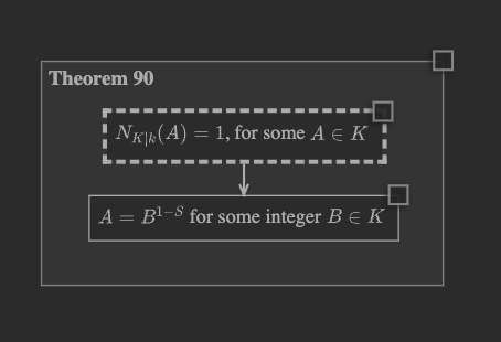
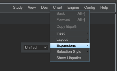
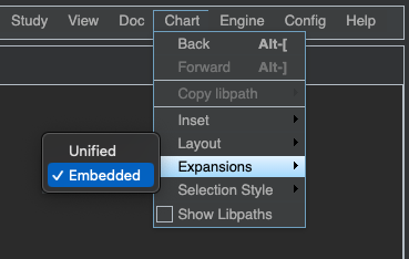
Go to the “Chart” menu, find “Expansions,” and make sure it is set to “Unified.”

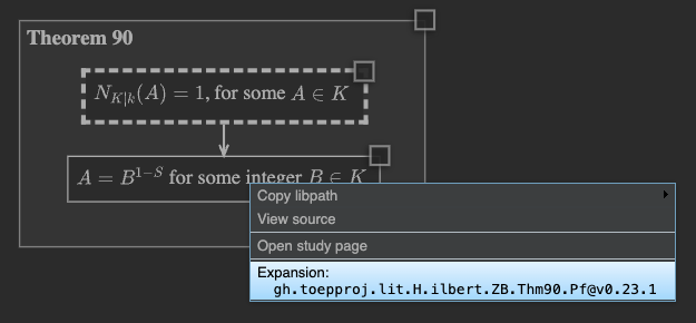
Then right-click the conclusion node in the theorem, and select the gh.toepproj.lit.H.ilbert.ZB.Thm90.Pf expansion to open the proof.

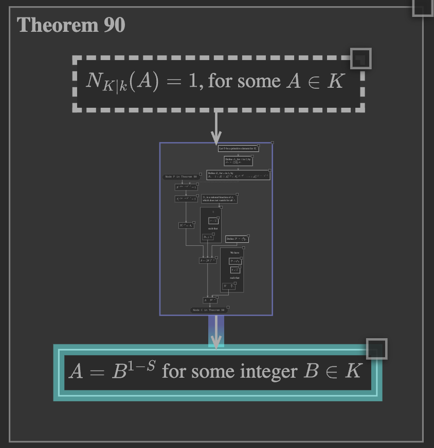
When the proof opens, we get a “unified” presentation, in which the nodes of the proof are drawn at the same scale as the nodes of the theorem. Notice also that there are edges connecting nodes of the theorem to nodes of the proof.

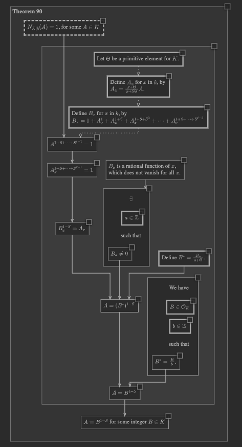
Zooming in and examining the proof, when we come to the node that says \(A_x^{1 + S + \cdots + S^{\ell - 1}} = 1\), we can right-click this node, and click to open the expansion gh.toepproj.ex.H.ilbert.ZB.Thm90.X2.

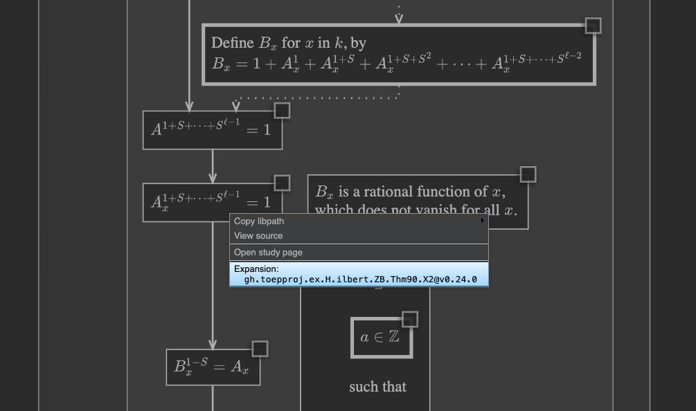
Again, since we’re in unified mode, room is made to insert the expansion at the same scale as the surrounding proof, and there are edges connecting proof nodes to expansion nodes.

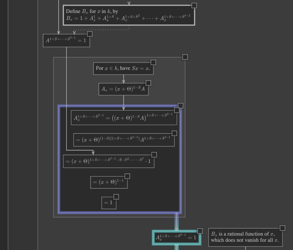
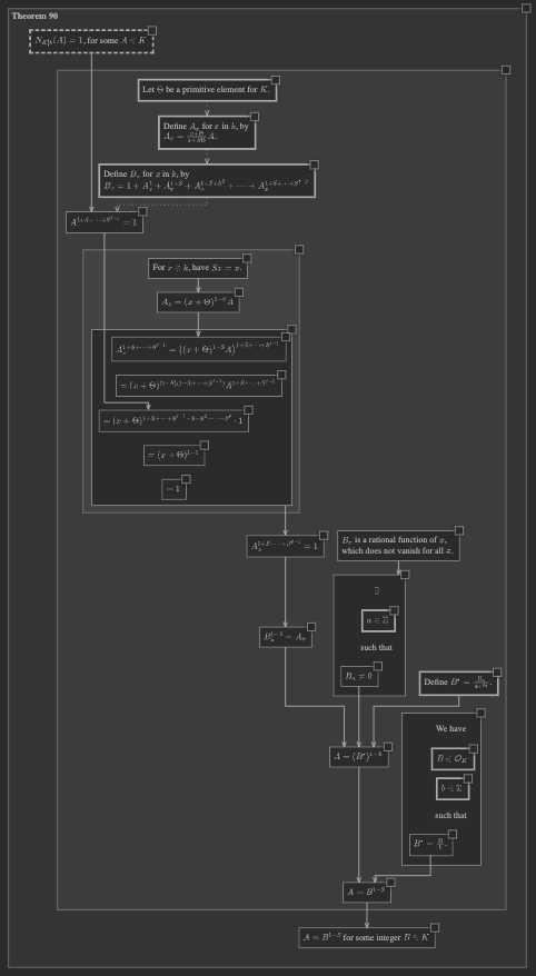
Zooming back out to the overview, we can see that our full chart has grown considerably in size, and all nodes are drawn at a single, unified scale.

Embedded mode

The idea of embedded mode is that expansions are scaled down and embedded into the deductions on which they expand. If expansion \(E\) expands on deduction \(D\), then \(E\) is drawn at a smaller scale, so that the whole of \(E\) is about as big as a single node of average size in \(D\).

Drawing expansions this way makes it so that you have to zoom in to read them. This can be thought of as a visual metaphor, representing expansions as “details.”

To see an example, we can go back to the same theorem we opened in PISE earlier. This time, be sure to go to the “Chart” menu, and under “Expansions” switch to “Embedded”.

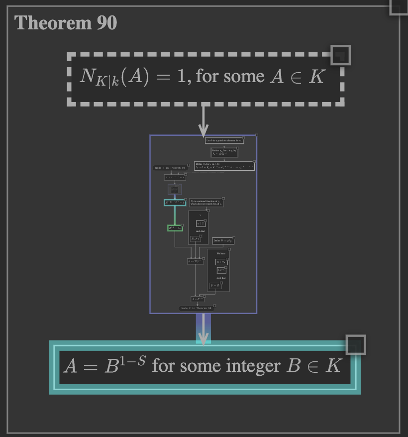
Then once again right-click the conclusion node of the theorem and open the proof. This time, the entire proof is scaled down and “embedded,” so that it is about as large as a single one of the theorem’s nodes.

We can zoom in, to make the proof readable.

Tip

Zoom using either Ctrl + mouse wheel, or pinch gesture on a multi-touch trackpad.

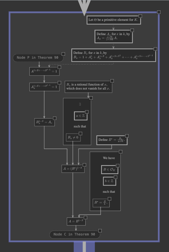
Notice that, in embedded mode, there are no edges connecting nodes of the theorem to nodes of the proof. Instead, you can see “ghost nodes” in the proof, representing nodes of the theorem. For example, find the one labeled, Node P in Theorem 90. If you hover your mouse over these ghost nodes, you can see a popup showing the node from the theorem.

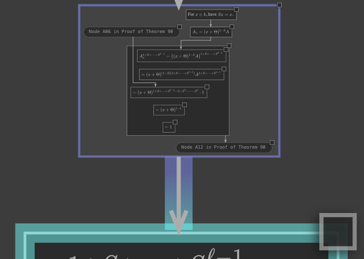
Next, once again locating the \(A_x^{1 + S + \cdots + S^{\ell - 1}} = 1\) node, right-click to open the gh.toepproj.ex.H.ilbert.ZB.Thm90.X2 expansion.

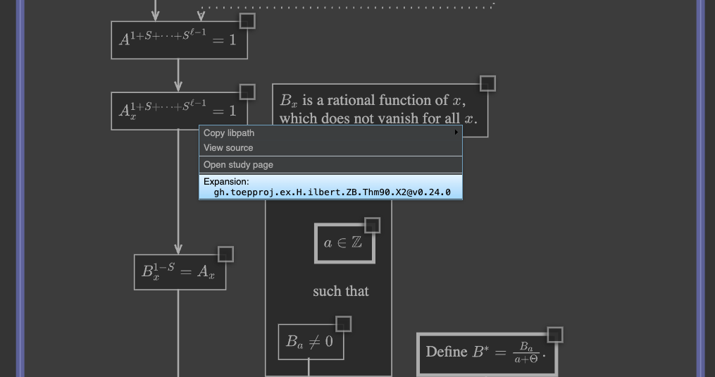
Again, embedded mode means the entire expansion is drawn about as large as a single one of the proof’s nodes:

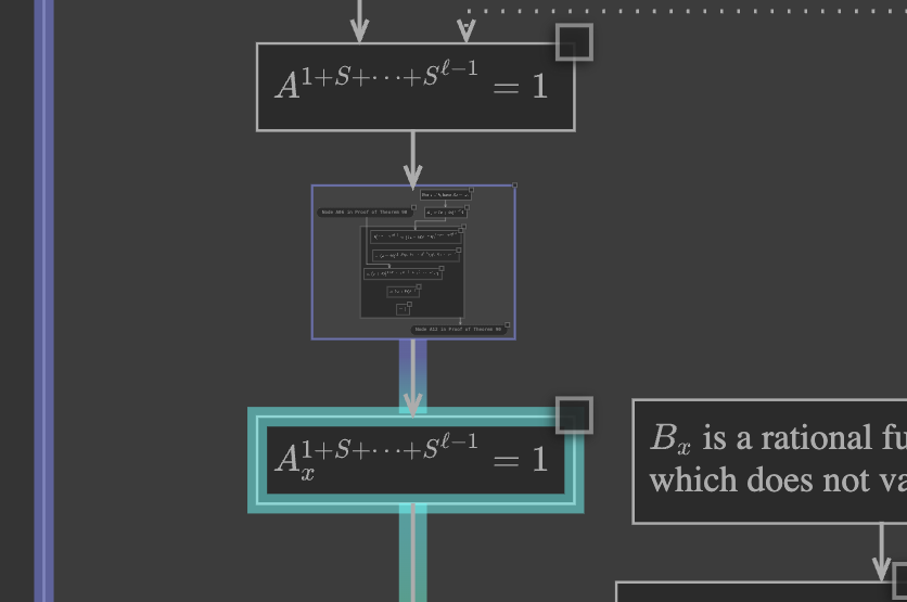
In this way, it is depicted as a “set of details,” which can help us achieve one step in the proof. If we are interested in those details, we can zoom in and study them:

Zooming back out to the overview, we find that the theorem is regular size, the proof is small, and the expansion is tiny, but visible.

Conclusion

You have learned to use both the unified and embedded expansion modes. Each has its advantages and disadvantages.

Unified mode keeps all nodes simultaneously legible, and allows them to connect to each other across expansion boundaries; however, more and more space is required, and the visual distinction between expansions and their surroundings is subtle, being marked only by the expansion’s outer boundary box.

Embedded mode visually emphasizes the distinction between an expansion and its surroundings, by scaling it down to make it look like “details.” This arrangement lets us zoom in if we are interested in those details, or stay zoomed out and let the expansion simply appear as an (illegible) “reminder” that further details are available. Embedded mode packs a lot into a small space, but nodes at different levels are not simultaneously legible, and we cannot draw edges connecting nodes across different levels.