Part 5: Doc Labels#
In Part 4: Doc Widgets, we used a doc widget to link from an annotation to a PDF. In this part, we’ll put a doc label on a node in a deduction, in order to make a link from that node to a PDF.
Open the document#
Start by opening the same PDF we worked with in Part 4: Doc Widgets. If it’s not still open, you can once again find the “Doc” menu in the toolbar at the top of the PISE window, select “Open PDF from the web…” and enter the URL:
https://resources.proofscape.org/cors/pdf/example/primes.pdf
Write deductions#
Let’s now build a representation of the results from the PDF, in the form of
Proofscape deductions. Open the file primes.pfsc from Part 4: Doc Widgets,
paste the following deductions into it at the end, and rebuild.
deduc Lem1 {

    asrt C {
        en = "
        Every composite number is divisible
        by some prime number.
        "
    }

    meson = "C"
}


deduc Thm2 {

    asrt C {
        en = "
        There are infinitely
        many prime numbers.
        "
    }

    meson = "C"
}


deduc Pf2 of Thm2.C {

    supp S10 {
        en = "
        Suppose there were only
        finitely many primes.
        "
    }

    intr I20 {
        en = "
        Let all the primes be
        $p_1, p_2, \ldots, p_n$.
        "
    }

    intr I30 {
        en = "
        Let $N = p_1 p_2 \cdots p_n + 1$.
        "
    }

    asrt A40 {
        en = "
        For all $i$, $N > p_i$.
        "
    }

    asrt A50 {
        en = "
        For all $i$, $N \neq p_i$.
        "
    }

    asrt A60 {
        en = "$N$ is composite"
    }

    exis E70 {
        intr I {
            en = "a prime number $p$"
        }
        asrt A {
            sy = "$p \mid N$"
        }
    }

    asrt A80 {
        sy = "$N \equiv 0 \mod p$"
    }

    asrt A90 {
        sy = "$N \equiv 1 \mod p$"
    }

    flse F100 contra S10 {}


    meson = "
    Suppose S10. Let I20. Let I30.
    Then A40, so A50, hence A60.
    Therefore E70, using Lem1.
    From E70.A get A80, but A90 by I30 and E70.I.
    Hence F100, by A80.
    Therefore Thm2.C.
    "
}
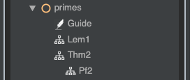
Once the build completes, the “Structure” tab in the sidebar should now
show that the primes module defines four objects:
the Guide annotation we defined in the last part,
plus the Lem1, Thm2, and Pf2 deductions we have just now added.
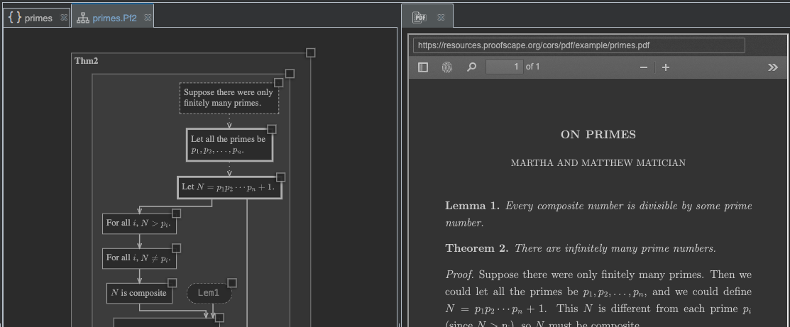
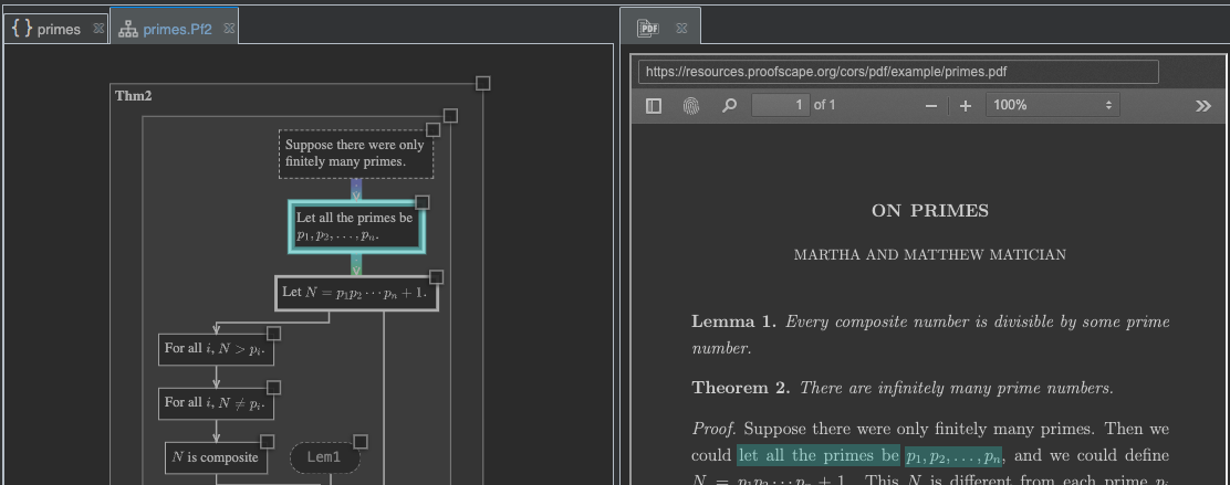
Double-click Pf2 to open a chart panel showing the proof, as well as the theorem
it proves.
As in Part 4: Doc Widgets, let’s set up our workspace with the PDF panel on the right, and the chart and source panels on the left.
Define a doc label#
We’re ready now to define a doc label on a node in our Pf2 deduction.
For our first example, we’ll define a label for node I20, which introduces
the primes \(p_1, p_2, \ldots, p_n\).
First, adjust the zoom level in your PDF panel to 100%.
Tip
If only the - and + buttons are visible in the center of the PDF panel toolbar, widen the panel until the zoom dropdown appears. Then you can see the zoom level.
Note
In general, it is fine to make PDF labels at any zoom level that matches the node sizes you want. In our present example, 100% happens to be the right level.
As you learned to do in Define a doc widget, switch the PDF panel into Box Selection mode. This time we’re going to draw two boxes, as shown here:
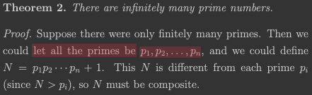
Although the gap between them is small, you should be able to see that one box covers just the words, “let all the primes be,” while the other covers the symbols “\(p_1, p_2, \ldots, p_n\)”.
Important
For the purposes of this tutorial, please draw the left-hand box first, then the right-hand box. In practice, any order will work, but for the instructions written below, this order is necessary.
When you’ve drawn the two boxes to your satisfaction (again, refer back to Define a doc widget for tips on drawing and adjusting boxes), double-click either box to open the combiner dialog.
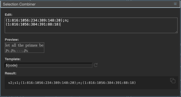
The “Edit” box at the top of the combiner dialog shows our two box definitions
(the numerical parts bounded by parentheses) as well as a newline command n;
that puts our second box on a second row. (See Box Combiner Codes.)
The layout visible in the “Preview” box is not bad at all, but let’s suppose we wanted to adjust it. In the “Edit” box, put your cursor at the start of the second line, and add the text,
x+27;y+2;
at the start of the line. By adding these two commands (one x-shift and one y-shift command), you have shifted the second box to the right, and slightly down.
Next, let’s use the “Template” box (see Using a template).
Since we already took the time to Define a doc info object in the last part,
which we called OnPrimes, we can now simply drop
doc = "OnPrimes#${code}"
into the “Template” box, to prepare the right label definition.
At this point, your combiner dialog should look something like this:
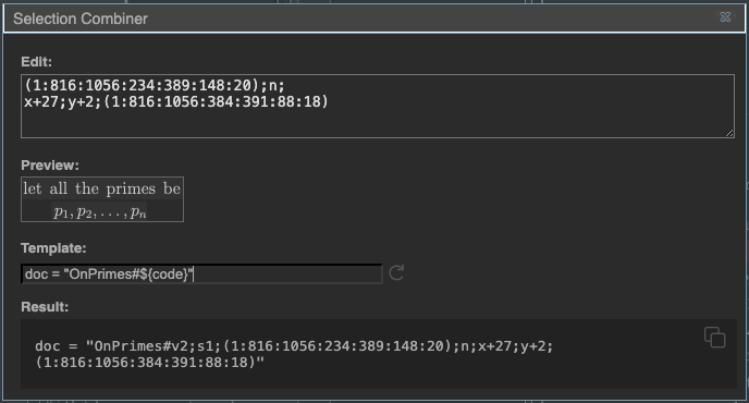
(except that your exact box codes may differ).
Finally, copy the full text from the “Result” box, close the combiner dialog,
and add the text into the definition of node I20 in the Pf2 deduction.
The full node definition should now look like this:
intr I20 {
    en = "
    Let all the primes be
    $p_1, p_2, \ldots, p_n$.
    "

    doc = "OnPrimes#v2;s1;(1:816:1056:233:389:148:19);n;x+27;y+2;(1:816:1056:385:393:87:16)"
}
Rebuild, and then switch back to the chart panel. Try clicking the node where we introduce the primes \(p_1, p_2, \ldots, p_n\), and the corresponding boxes in the PDF should now light up.
Show a doc label on a node#
In our current definition for node I20 (Listing 13),
we have defined two labels: one TeX label, and one doc label.
Try now commenting out the TeX label, so that your node definition looks like this:
intr I20 {
    #en = "
    #Let all the primes be
    #$p_1, p_2, \ldots, p_n$.
    #"

    doc = "OnPrimes#v2;s1;(1:816:1056:233:389:148:19);n;x+27;y+2;(1:816:1056:385:393:87:16)"
}
Then rebuild, and switch back to the chart panel. You should be able to see that the label on this node now looks a bit different.
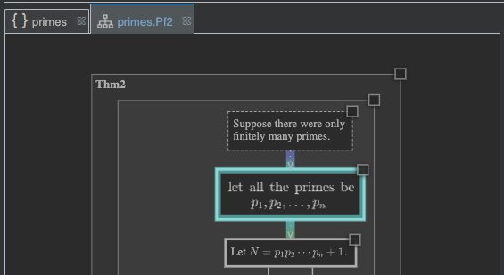
It is showing the exact label defined by the boxes
in the PDF. The PDF has to be present for this to work. (You can try closing both the PDF
and the chart panel, then re-opening the Pf2 deduc to see what happens when the PDF is
not present.)
Define many doc labels#
In Listing 14,
we have defined a doc label on every node of Pf2.
Replace your existing definition of Pf2 with this version, and rebuild.
As you may notice in Listing 14,
we defined docInfo at the top of
the deduction, and in none of our doc labels do we make any further reference
to the OnPrimes document.
By defining docInfo in the deduction, we indicated the default document to
which any doc labels on its nodes now automatically refer.
See Format options.
Tip
If for some reason you need a single deduction to refer to two different docs, you can still define a default doc. Just make explicit reference to the second doc in those labels that want to point to it.
deduc Pf2 of Thm2.C {

    docInfo = OnPrimes

    supp S10 {
        en = "
        Suppose there were only
        finitely many primes.
        "

        doc = "v2;s1;(1:816:1056:237:365:172:20);n;(1:816:1056:410:364:148:21)"
    }

    intr I20 {
        en = "
        Let all the primes be
        $p_1, p_2, \ldots, p_n$.
        "

        doc = "v2;s1;(1:816:1056:233:389:148:19);n;x+27;y+2;(1:816:1056:385:393:87:16)"
    }

    intr I30 {
        en = "
        Let $N = p_1 p_2 \cdots p_n + 1$.
        "

        doc = "v2;s1;(1:816:1056:581:387:46:22);n;(1:816:1056:188:411:144:21)"
    }

    asrt A40 {
        en = "
        For all $i$, $N > p_i$.
        "

        doc = "v2;s1;(1:816:1056:236:434:48:24)"
    }

    asrt A50 {
        en = "
        For all $i$, $N \neq p_i$.
        "

        doc = "v2;s1;(1:816:1056:387:411:135:22);n;(1:816:1056:525:412:102:23)"
    }

    asrt A60 {
        en = "$N$ is composite"

        doc = "v2;s1;(1:816:1056:317:436:150:20)"
    }

    exis E70 {
        intr I {
            en = "a prime number $p$"

            doc = "v2;s1;z1;(1:816:1056:506:461:94:22)"
        }
        asrt A {
            sy = "$p \mid N$"

            doc = "v2;s1;z2;(1:816:1056:346:459:20:21);(1:816:1056:424:459:81:23);x+1;y+3;(1:816:1056:588:462:12:19)"
        }

        doc = "v2;s1;(1:816:1056:347:459:252:24)"
    }

    asrt A80 {
        sy = "$N \equiv 0 \mod p$"

        doc = "v2;s1;(1:816:1056:340:484:101:22)"
    }

    asrt A90 {
        sy = "$N \equiv 1 \mod p$"

        doc = "v2;s1;(1:816:1056:266:509:100:22)"
    }

    flse F100 contra S10 {
        doc = "v2;s1;(1:816:1056:375:510:130:20)"
    }


    meson = "
    Suppose S10. Let I20. Let I30.
    Then A40, so A50, hence A60.
    Therefore E70, using Lem1.
    From E70.A get A80, but A90 by I30 and E70.I.
    Hence F100, by A80.
    Therefore Thm2.C.
    "
}
After rebuilding, try once again clicking through the nodes in the chart, as well as hovering your mouse over all the lines in the proof in the PDF, and clicking highlights as they come up.
Note
You may notice the overlap of the highlights we selected for labels in the existential
node E70 and its subnodes E70.I and E70.A. In order to make all three labels
accessible from the PDF, we manually added z-index commands to the doc labels for
E70.I and E70.A. If you examine their doc label codes in Listing 14,
you will find the commands z1; and z2;.
This works just like the CSS z-index property. The default level
is 0, and elements with higher z-index lie above those with lower index.
In many cases, PISE will automatically elevate highlights to make them accessible, and you do not need to use manual z-index commands in such cases. For example, this takes place whenever one highlight is contained entirely within another.
In practice, it’s a good idea to add manual z-index commands only if you find that a highlight is actually inaccessible.
Reuse a doc label in an annotation#
Once you have defined a doc label on a node, you can then reuse it from a doc widget in an annotation or Sphinx page.
In primes.pfsc, go back to the Guide annotation we wrote in Part 4: Doc Widgets,
and change the value in the sel field of the final doc widget to Pf2.A90.
The last three lines of the annotation should now appear as in Listing 15.
} and <doc:>[to $1$]{
    sel: Pf2.A90
} mod some prime $p$, and this contradiction completes the proof.
Note
There are no quotation marks around Pf2.A90 in Listing 15
because this is not a string, it is a libpath as a primitive.
Now rebuild, and open the Guide annotation. You should find that the final doc widget still
highlights the desired selection in the PDF. This works because node A90 in Pf2 is pointing
to the same step in the proof.
Reuse doc labels whenever possible#
In the last section, we made a doc widget copy its reference from a node. It’s a good idea to do this whenever possible, as it fits into a logical workflow:
First represent a proof in the form of a Proofscape deduction, adding doc labels wherever appropriate.
Then write commentary on the proof, in the form of annotations or Sphinx pages. If you use doc widgets, copy the references from the corresponding nodes.
Among the advantages of working this way are that:
Multiple authors may each want to write their own commentary on the proof, and it makes sense for all commentators to reuse the same deductions and doc refs.
Highlights work better when they are reused, instead of being redundant and overlapping.
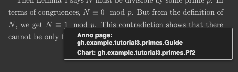
In order to illustrate the second point, about reuse being better than overlap, try hovering your mouse over the congruence \(N \equiv 1 \mod p\) in the PDF, for which we reused a highlight in the last section.
You should notice that the mouse cursor takes on a new form, suggesting a context menu. When you click (left-click, not right-), you should see a menu from which you can choose either the annotation or the chart, each of which has made a reference to this point in the proof. Go ahead and try each option.
Tip
For more about the ways in which different content panels can be linked to each other, see Linking.
By contrast, try now hovering your mouse over the opening sentence of the proof, “Suppose there were only finitely many primes,” in the PDF panel. Depending on how you drew your boxes earlier, you may find that clicking here does nothing. What we have are two highlights, mostly overlapping, and PISE is trying to draw them both, and find each one an independent space where it can be clicked.
In order to remedy the situation, let’s now redo all the remaining doc widgets in our Guide annotation,
so that each one now references the appropriate node from the Pf2 deduction. When you’re done, the annotation
should be as in Listing 16.
anno Guide @@@
# Key Ideas

In the proof of the infinitude of primes, the key construction is
<doc:>[the number $N$]{
    sel: Pf2.I30,
}.
Having <doc:>[supposed]{
    sel: Pf2.S10
} there were only finitely many primes, we conclude that $N$
must be congruent both <doc:>[to $0$]{
    sel: Pf2.A80
} and <doc:>[to $1$]{
    sel: Pf2.A90
} mod some prime $p$, and this contradiction completes the proof.
@@@
Rebuild one last time, and then go back to the PDF panel and try using the highlights again. This time, you should find that all reused highlights are clickable and functional.
Summary#
You have learned how to:
Add a doc label to a node
Show a doc label (by defining no TeX label)
Define a default doc, using the
docInfofield in a deductionReuse a node’s doc label in a doc widget in an annotation